Applying DNN Approximations with ApproxTuner
In this tutorial, we’ll apply autotuning on a DNN (compiled as a binary) to find approximation choices (configurations), and profile the selected configurations to get real performance on device. The result will be a tradeoff curve between the model’s classification accuracy and performance improvement (speedup); ApproxTuner will automatically generate a figure of this tradeoff curve.
Make sure you have read through the previous tutorial first.
Compiling a Tuner Binary
The previous binary is used for inference purpose.
To use the autotuner, we need a slightly different binary that can talk with the tuner.
The following code is almost identical to the last code block,
but it adds target="hpvm_tensor_inspect" to ModelExporter,
to require an autotuner binary.
It also doesn’t require a conf_file argument.
from pathlib import Path

import torch
from pytorch import dnn  # Defined at `hpvm/benchmarks/dnn_benchmarks/pytorch/dnn`
from torch2hpvm import BinDataset, ModelExporter
from torch.nn import Module

data_dir = Path("./model_params/vgg16_cifar10")
dataset_shape = 5000, 3, 32, 32  # NCHW format.
tuneset = BinDataset(data_dir / "tune_input.bin", data_dir / "tune_labels.bin", dataset_shape)
testset = BinDataset(data_dir / "test_input.bin", data_dir / "test_labels.bin", dataset_shape)

model: Module = dnn.VGG16Cifar10()
checkpoint = "model_params/pytorch/vgg16_cifar10.pth.tar"
model.load_state_dict(torch.load(checkpoint))

tuner_output_dir = Path("./vgg16_cifar10_tuner")
tuner_build_dir = tuner_output_dir / "build"
tuner_binary = tuner_build_dir / "vgg16_cifar10"
exporter = ModelExporter(model, tuneset, testset, tuner_output_dir, target="hpvm_tensor_inspect")
metadata_file = tuner_output_dir / exporter.metadata_file_name
exporter.generate(batch_size=500).compile(tuner_binary, tuner_build_dir)
This binary is generated at vgg16_cifar10_tuner/build/vgg16_cifar10.
It waits for autotuner signal and doesn’t run on its own, so don’t run it by yourself.
Instead, import the tuner predtuner,
and tell the path to the binary (tuner_binary) to the tuner to use it:
from predtuner import PipedBinaryApp, config_pylogger

# Set up logger to put log file here
msg_logger = config_pylogger(output_dir="./", verbose=True)

# Create a `PipedBinaryApp` that communicates with HPVM bin.
# "TestHPVMApp" is an identifier of this app (used in logging, etc.) and can be anything.
# Other arguments:
#   base_dir: which directory to run binary in (default: the dir the binary is in)
#   qos_relpath: the name of accuracy file generated by the binary.
#     Defaults to "final_accuracy". For HPVM apps this shouldn't change.
#   model_storage_folder: where to put saved P1/P2 models.
app = PipedBinaryApp(
  "TestHPVMApp",
  tuner_binary,
  metadata_file,
  # Where to serialize prediction models if they are used
  # For example, if you use p1 (see below), this will leave you a
  # tuner_results/vgg16_cifar10/p1.pkl
  # which can be quickly reloaded the next time you do tuning with
  model_storage_folder="tuner_results/vgg16_cifar10",
)
tuner = app.get_tuner()
tuner.tune(
  max_iter=1000,  # Number of iterations in tuning. In practice, use at least 5000, or 10000.
  qos_tuner_threshold=3.0,  # QoS threshold to guide tuner into
  qos_keep_threshold=3.0,  # QoS threshold for which we actually keep the configurations
  is_threshold_relative=True,  # Thresholds are relative to baseline -- baseline_acc - 3.0
  take_best_n=50,  # Take the best 50 configurations,
  cost_model="cost_linear",  # Use linear performance predictor
  qos_model="qos_p1",  # Use P1 QoS predictor
)
fig = tuner.plot_configs(show_qos_loss=True)
fig.savefig("configs.png", dpi=300)
app.dump_hpvm_configs(tuner.best_configs, "hpvm_confs.txt")
Note that the performance shown here is estimated.
cost_model="cost_linear"estimates the performance of a configuration using the FLOPs of each operator and the FLOPs reduction of each approximation. The next section talks about profiling (on a different machine), which shows the real performance.If you are tuning on the end device that you wish to run the inference on, (which is a rare case), then removing this argument will make the tuner measure real performance instead. In that case, you may skip the profiling step.
Arguments
cost_modelandqos_modelcontrols the models used in tuning. No models are used when the argument is omitted. For example, you can do an empirical tuning run by removingqos_model="qos_p1".The
metadata_filevariable passed to the tuner is the path to a metadata file generated by the frontend; the tuner reads it to know how many operators are there and what are the applicable knobs to each operator.
This tuning process should take a few minutes to half an hour, depending on your GPU performance. After the tuning finishes, the tuner will
generate a figure showing the performance-accuracy tradeoff, at
./configs.png, andsave the HPVM config format (write-only) at
./hpvm_confs.txt.
It is also possible to save the configuration in other formats (see the predtuner documentation).
Profiling the Configurations on Target Device
We will use hpvm_profiler (a Python package) for profiling the ./hpvm_confs.txt
we obtained in the tuning step.
The profiler uses the plain binary generated in the beginning (
./vgg16_cifar10/build/vgg16_cifar10) instead of the tuner binary.Note that you may want to run this profiling step on the edge device where the performance gain is desired. As the compiled binary is usually not compatible across architectures, you need to install HPVM on the edge device and recompile the model. You may also want to skip Python packages in the installation to reduce some constraints on Python version and Python packages.
Also note that currently, the approximation implementations in the tensor runtime are tuned for Jetson TX2, and speedup may be less for other architectures.
from hpvm_profiler import plot_hpvm_configs, profile_config_file

# Set `target_binary` to the path of the plain binary.
target_binary = "./vgg16_cifar10/build/vgg16_cifar10"
# Set `config_file` to the config file produced in tuning, such as "hpvm_confs.txt".
config_file = "hpvm_confs.txt"
out_config_file = "hpvm_confs_profiled.txt"
profile_config_file(target_binary, config_file, out_config_file)
plot_hpvm_configs(out_config_file, "configs_profiled.png")
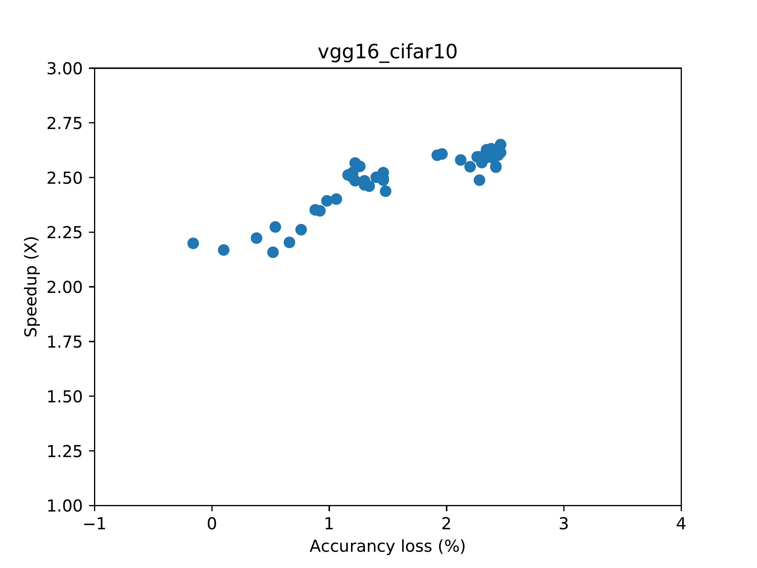
hpvm_confs_profiled.txt contains the profiled configurations in HPVM format,
while configs_profiled.png shows the final performance-accuracy tradeoff curve.
An example of configs_profiled.png looks like this (proportion of your image may be different):